The Most Basics of Neural Networks

This blog post will be about the most basics of neural networks, for absolute beginners.

You've heard about things like ChatGPT, LlaMa, Midjourney, Dall-E, and Stable Diffusion. But have you ever wondered how exactly does they work? In this blog series, I will explain the neural network, from the absolute basics to advanced, from simple fully-connected networks to Transformers, Quantum Neural Networks, and Graph Neural Networks. If you encountered any questions, feel free to ask by directly through my email or by Discord!

Prerequisites

• Basic Maths
• Basic Python

Aims

1. Understand the neurons and neural networks
2. Understand the use of neural networks
3. Understand forward pass, loss function, backward pass, and weight update

Introduction

“I think the brain is essentially a computer and consciousness is like a computer program. It will cease to run when the computer is turned off. Theoretically, it could be re-created on a neural network, but that would be very difficult, as it would require all one's memories.” ~ Stephen Hawking

Important Concepts

Neurons and Neural Networks

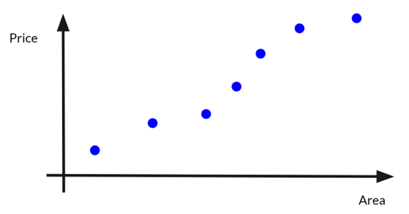
Imagine you are making a system to predict property prices. How would you implement such a system? Maybe it will take the different factors of a property (e.g. size, height, view, surrounding environment, etc.) to calculate the price and outputs it. But how can you calculate the price based on these inputs (factors)?

Let’s simplify the problem and assume there is only one factor: the size (area) of the property. Let’s plot a graph with the area on the x-axis, price on the y-axis:

Then we can draw a straight fit line on the graph to relate all the data points:

tip

Note that the fit line may not pass through all/any data points!

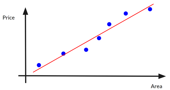
How can you represent the fit line in maths? We can use a simple linear function:

$$f(x) = wx + b$$

Where w is the weight (the steepness of the linear), b is the bias (the y-intercept, or height of the line). In fact, we can represent any straight line on a two-dimensional Cartesian coordinate space and any linear functions with one variable with this function. In the neural network, this function is the simplest form of a neuron. But what is a neuron? This is an anatomy of a human neuron cell:

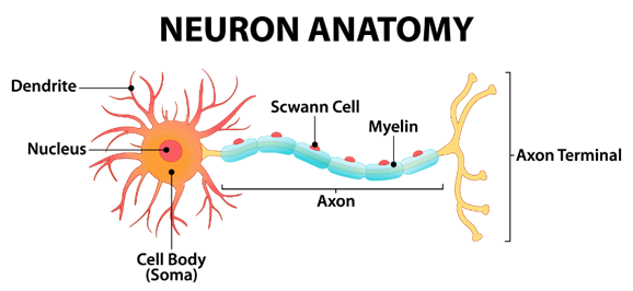
The dendrites receive the signals, the cell processes the signals, and the axon terminals send the signals to other neuron cells. By connecting 86 billion of these cells, it forms your brain. We can simulate a neuron in maths with the following function:

$$f(x_1, x_2, x_3, x_4, \ldots) = w_1 x_1 + w_2 x_2 + w_3 x_3 + w_4 x_4 + \cdots + b$$

The multiple weights represent the “importance” of each of the different input x. The b is still the bias. Here’s another diagram to understand the neuron:

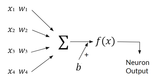
So, for example, the multiple x can be the different factors of the property, and the weights are parameters that you can tune, representing the importance of that factor contributing to the final price. Wait, what is the f(x) in the above diagram? It is an Activation Function. Its purpose is to introduce non-linearity into the neural network as combining linear functions can only result in a linear function:

Let $f(x) = w_1 x + b_1$, $g(x) = w_2 x + b_2$, then $h(x) = g(f(x))$:

$$h(x) = g(f(x)) = w_2 (w_1 x + b_1) + b_2$$ $$h(x) = w_2 w_1 x + w_2 b_1 + b_2$$

Let $a = w_2 w_1$ and $c = w_2 b_1 + b_2$, then:

$$h(x) = ax + c$$

Which is a straight line on the graph. But by adding activation functions in between, e.g. $h(x)=g(a(f(x)))$, where $a$ is the activation function, we can create a non-linear (broadly speaking not a straight line on the graph) function or network. Some common activation functions include ReLU, Sigmoid, Tanh, LeakyReLU, GELU, and Softmax. The details of the activation function will be talked about in later blog posts.

By combining and connecting multiple neurons in an orderly manner, you get a neural network. Below is a diagram of a neural network which you’ve probably seen before:

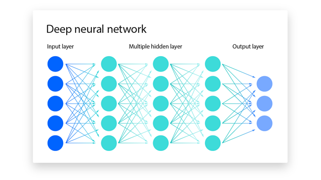
Each circle (node) in the neural network represents a neuron. Each neuron in the input layer processes a single number and each neuron in the output layer outputs a single number. Neural networks are universal function approximators.

info

Note that while the neurons in the hidden layer may seem to have multiple outputs, the outputs are the same.

Training of neural networks

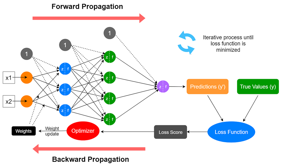
However, how can you calculate the weights and biases given x and y? Below are the processes of training a neural network to find the optimal weights and biases:

1. Initialize the weights and biases using random numbers with normal or uniform distribution.
2. Forward pass: Run the model with the input x, and get the model output y.
3. Compute loss: Compare the model-output y with the real targeted y and calculate the difference using a loss function.
4. Backpropagation/backward pass: Calculate the gradients of each parameter (weight or bias) using gradient descent with partial derivative. Which means how the output of the model changes with that parameter changing.
5. Update parameters: Update the parameters using optimizers based on the gradients calculated and the given learning rate hyperparameter (usually between 1e-2 to 1e-6).
6. Repeat Step 2 to 5 with different x and y until the loss is good enough.

Code Implementations

A simple neural network with PyTorch

Let’s consider a simple formula: y=3x+1. Given an array of x and array of the corresponding y, find 3 and 1 (the weight and the bias). Run the following codes in Google Colab for simplicity.

import torch # main library
import torch.nn as nn # neural network modules and functions
import torch.optim as optim # optimizers for neural networks
import matplotlib.pyplot as plt # plotting for analysing the loss

torch.manual_seed(69) # define a manual seed so the results are reproducible

Define the data x and y:

x = torch.tensor([0, 1, 2, 3, 4, 5, 6, 7, 8, 9, 10], dtype=torch.float32)
y = 3*x + 1

print(x.tolist())
print(y.tolist())

Define the model, loss function, and optimizer:

model = nn.Linear(1, 1) # a single neuron
criterion = nn.MSELoss() # Mean squared error (MSE) loss function
optimizer = optim.SGD(model.parameters(), lr=1e-4) # Stochastic Gradient Descent (SGD) optimizer

Training Loop:

epochs = 100
losses = []
for i in range(epochs):
    for iter_x, iter_y in zip(x, y):
        iter_x = iter_x.unsqueeze(0) # add another dimension at the end
        iter_y = iter_y.unsqueeze(0) # same
        optimizer.zero_grad() # zero the gradients
        output = model(iter_x) # Forward pass
        loss = criterion(output, iter_y) # Compute Loss
        loss.backward() # Backward pass
        optimizer.step() # Update parameters
        print(f"Epoch: {i}/{epochs}, Loss: {loss.item()}")
        losses.append(loss.item())

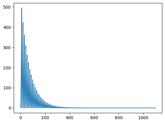
Final loss: 0.0001777520083123818

Plot the loss graph:

plt.plot(losses)
plt.show() # Plot the loss graph

Loss Graph:

Test the model:

for name, param in model.named_parameters():
    print(name, param) # Inspect the weight and bias

n = 100 # input x
x = torch.tensor([n], dtype=torch.float32) # convert to tensor
y = model(x) # Forward pass
print(y)

Follow-up Tasks

1. Experiment with different learning rates and epochs and see how it affects the training result.
2. Enlarge the dataset (lengthen the x tensor), does it improve the model?
3. Experiment with a more complex function than y=3x+1 such as y=x^2. Does it work? If it doesn’t work, how can you solve this issue?
4. How can you make the training faster without changing the hardware, data and the model?

Feel free to send me an email for your solutions to the above tasks!