Post-hackathon analysis of Efficient Gaussian State Preparation

Post-hackathon analysis of Our Solution at MIT iQuHACK 2025

Introduction

In a previous blog post, we presented our MIT iQuHACK 2025 solution for preparing a Gaussian state on a quantum computer using a two-step approach:

1. Bitwise (product) state preparation via RY rotations with angles chosen to induce exponential decay per qubit.
2. Approximate Quantum Fourier Transform (QFT) with pruning of small-angle controlled-phase gates to keep the circuit cost nearly linear in the number of qubits.

By testing it on the Classiq platform, We demonstrated that this method yields an acceptably small mean-squared error (MSE) while maintaining scalability. After the hackathon, we continued investigating this technique—particularly, how well it accommodates different resolutions (number of qubits) and how the shape of the Gaussian (controlled by the parameter $\sigma$ or EXP_RATE) affects fidelity.

This follow-up blog post summarizes these explorations, includes additional visualizations, and discusses next steps such as parameter optimization and potential integration into quantum machine learning (QML) tasks.

Testing at Different Resolutions

One of the first post-hackathon experiments was to test the same circuit design at different resolutions $(r=5 \text{ to } 16)$. Here is are the results of these runs:

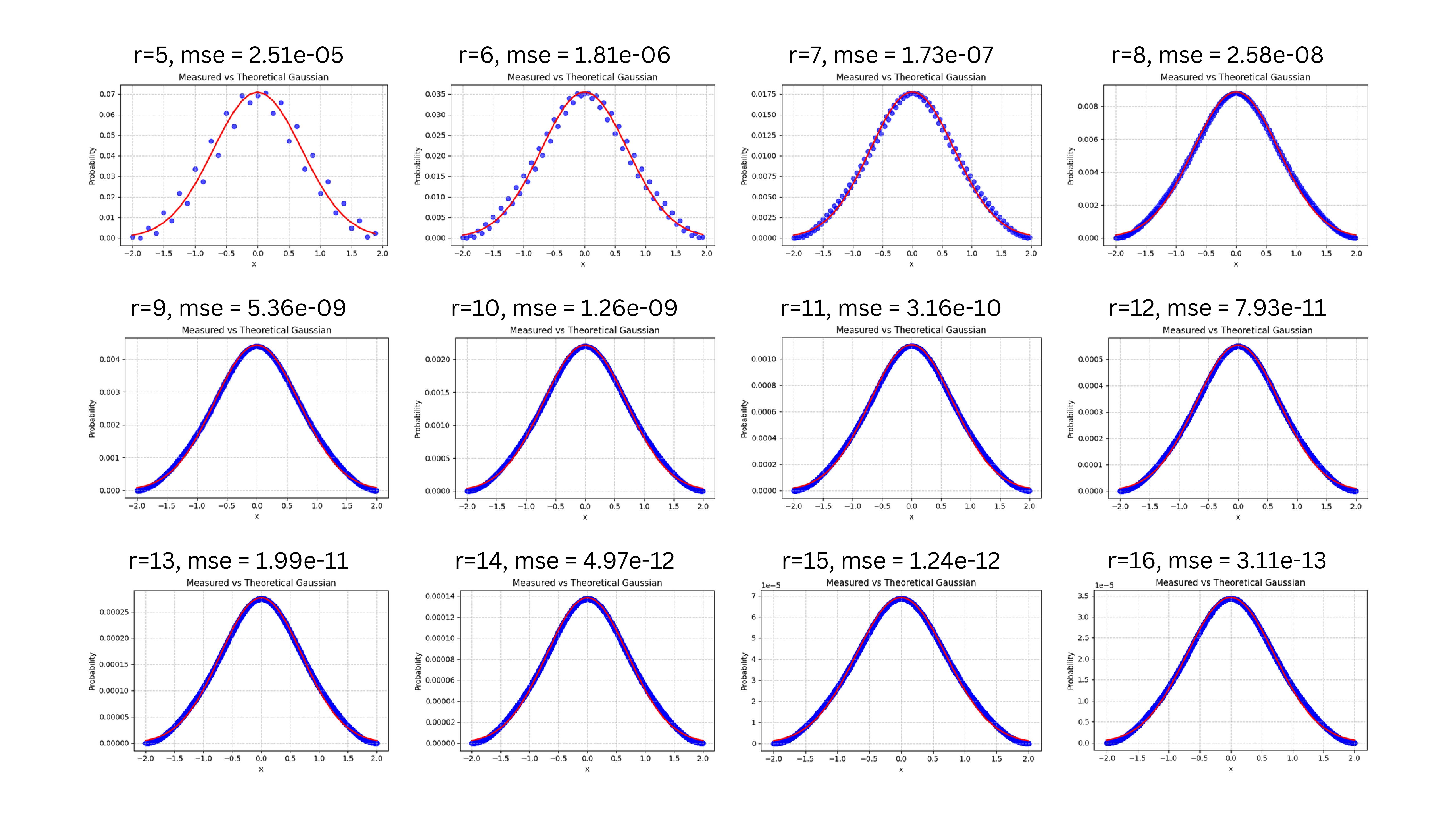
The circuit structure and parameters (apart from changing the qubit count) remain the same for each experiment. As expected, as $r$ grows, the MSE improves because a higher-resolution grid captures the discrete Gaussian more finely. This is consistent with our original hackathon findings: the approximate QFT approach benefits from increased dimensionality, so long as we can handle the gate overhead (mitigated by pruning small-angle controlled-phase gates).

Varying $\sigma$ and the “Shoulder” Phenomenon

Another goal was to see how well the circuit adapts to different Gaussian widths, controlled by $\sigma$. Recall that in the hackathon, we mostly focused on a single value $\sigma$. Extending that to arbitrary $\sigma$ values unveiled an interesting “shoulder” phenomenon on both tails of the Gaussian for certain $\sigma$ ranges.

Below is a short video (different_sigma.mp4) illustrating how the amplitude distribution transitions as $\sigma$ varies from $1 \text{ to } 5$. Notice that for significantly different $\sigma$ from unity, the circuit’s approximation is less accurate at the tails:

We suspect the cause is that our initial RY-based product state and the single global QFT are not fully flexible in matching the shape of a “true” Gaussian when $\sigma$ deviates substantially from 1. This prompts us to investigate the deeper mathematical models involved in the quantum circuit in order to fully understand the "shoulder" problem.

Plotting MSE as a Function of $\sigma$

To quantify how the circuit’s fidelity changes with $\sigma$, we let MSE as a function of $\sigma$ and measured the MSE for a range of $\sigma$ values. Surprisingly, the region where MSE changes the least seems to lie around $\sigma \approx e$. We also calculated $\frac{d\,\mathrm{MSE}}{d\,\sigma}$ and observed that its behavior is most favorable near $\sigma=e$. The reason might be tied to how the approximate QFT’s discrete frequencies interact with the bitwise angles in the initial state, further investigation is required.

Below is the plot of $\mathrm{MSE}(\sigma)$:

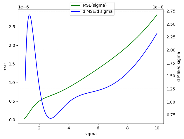
Figure: MSE versus $\sigma$. At $\sigma = e$, the slope $\frac{d\,\mathrm{MSE}}{d\,\sigma}$ is notably small, suggesting a “sweet spot” for this particular parameterization.

Preliminary Real-Hardware Tests on IBM Brisbane

To explore the robustness of our approach under realistic conditions, we ran the circuit on IBM's Brisbane quantum device through the Classiq platform.

We employed 5 qubits and collected 5000 shots. Despite hardware noise and inevitable gate errors, the measured distribution still resembled a Gaussian-like shape in the histogram of outcomes. Below is a figure depicting the measured distribution:

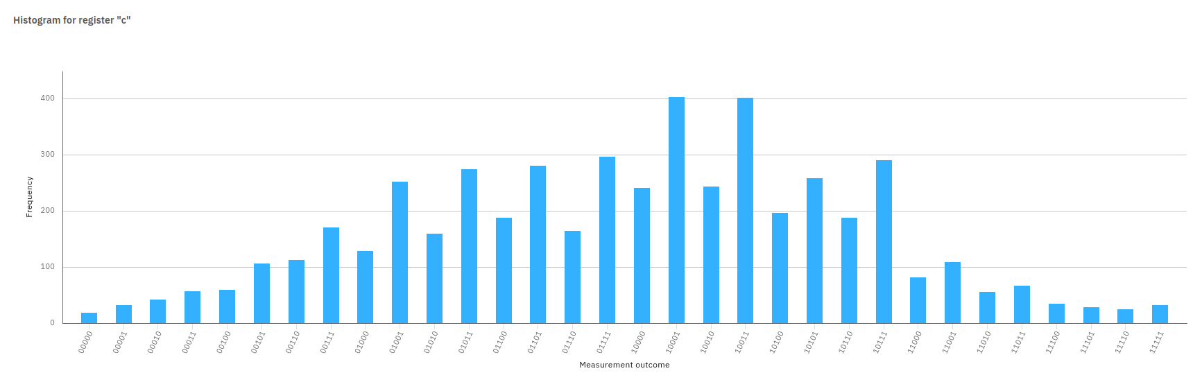
Figure: Measurement outcomes from IBM Brisbane with 5 qubits. A semblance of the Gaussian shape persists, though slightly distorted.

When we extended the circuit to 6 qubits or more, however, the noise effects amplified, and the Gaussian shape effectively vanished. This significant distortion suggests that higher qubit counts on current hardware require either more robust error mitigation or further refinements of the circuit to tolerate noise. We plan to investigate specialized noise-adaptive strategies or gate-error mitigation to see if we can preserve the Gaussian profile beyond 5 qubits.

Ongoing Directions and Next Steps

1. Adaptive Parameter Tuning

Our circuit still uses the same bitwise angle formula from the hackathon:

$$\theta_i = 2\,\arctan\bigl(e^{-i^2/(\frac{2\sigma^2}{5})}\bigr).$$

However, it might be possible to add a small correction term per qubit or introduce global phase factors such that the QFT outcome better fits a broader range of $\sigma$. This approach would entail optimizing angles for a given “target $\sigma$” to minimize MSE, akin to a small classical optimization loop.

2. Further Mathematical Analysis

Further mathematical analysis and modelling is required to understand the nature of the quantum circuit more completely, which is a fundamental step in solving problems like the "shoulder" phenomenom for arbitrary $\sigma$ and also explaning parameters like dividing by $\sqrt{5}$ in angle calculation.

3. Improved Approximate QFT Pruning

While the approximate QFT prunes CPhase gates with angles below a certain threshold, that threshold is static. We might allow a flexible threshold that depends on the qubit index (or a local cost function), further improving trade-offs between circuit depth and fidelity.

4. Integration into QML

A key motivation for Gaussian state preparation is quantum machine learning—e.g., embedding classical data or forming distribution-based feature maps. We performed a preliminary integration into a QML algorithm and observed some notable gains. Refinements, or a deeper synergy with QML-based cost functions, may achieve bigger improvements.

5. Real-Hardware Trials

All these simulations were performed in ideal, noiseless environments. Our initial tests on IBM Brisbane (5 qubits) demonstrate partial success, but the shape deteriorates at 6 qubits. Continued investigation of error mitigation, calibration, or noise-adaptive circuit designs could help preserve the Gaussian profile at larger scales.

6. Library Integration

We plan to provide a tutorial or example for approximate-QFT plus product-state preparation in the Classiq Library, demonstrating how to reduce gate counts for large resolutions.

Conclusion

Our post-hackathon exploration reaffirms that approximate QFT-based Gaussian state preparation is both scalable and flexible—but it also shows interesting parameter-dependent artifacts that warrant deeper analysis. By plotting $\mathrm{MSE}(\sigma)$ and visualizing amplitude profiles across resolutions and $\sigma$ values, we have pinpointed where the method remains robust and where further refinements are needed.

we look forward to further collaborations with Classiq and more thorough mathematical investigations to refine this approach. Stay tuned for additional results on parameter optimization, possible integration into Classiq’s library, and explorations of real-device performance.

Acknowledgements

I would like to express my sincere gratitude to Classiq for providing the platform and resources that enabled the successful completion of this research. Their innovative approach to quantum circuit design has been important in improving my understanding of quantum algorithms.

Furthermore, I acknowledge the support from the Classiq team and the vibrant community whose discussions and shared knowledge have been invaluable. A special thanks to Nadav Ben-Ami for his continuous guidance, encouragement, and insightful feedback throughout the research process. The original implementation of this work can be found in the Classiq Library repository, where further contributions and collaborations are warmly welcomed. I encourage anyone interested to explore, provide feedback, or contribute to the ongoing development.

As always, questions and feedback are welcome! I invite interested readers to connect and discuss further with us on my LinkedIn or Classiq's LinkedIn. I look forward to engaging conversations and future opportunities to collaborate within the growing field of quantum computing.

Stay tuned for the third blog post, where we will discuss about the underlying mathematical framework and share our latest progress on how to avoid the "shoulder" problem!