Introduction to Quantum Computing

The basics of quantum computing and some hands-on trying.

Prerequisites

• Basic Maths — linear algebra
• Basic quantum mechanics concepts — Superposition, the Uncertainty Principle, and Entanglement
• Basic Python
• Imagination power

Quantum Mechanics

“The mathematical framework of quantum theory has passed countless successful tests and is now universally accepted as a consistent and accurate description of all atomic phenomena.” ~ Erwin Schrödinger

We will not be talking about the advanced maths or concepts of quantum mechanics in this blog post, such as the Uncertainty Principle or the Schrödinger Equation, but I'll assume you know the main principles of Quantum Mechanics, including Superposition, Wave-Particle Duality, the Uncertainty Principle, and Entanglement. The concept of qubits and quantum circuits gates will be explained below.

Qubits

In normal semiconductor computers, each "bit" can only represent two values: 0 and 1, which can be used in calculations as low and high voltage. However, in quantum computers, "qubits" (quantum bit) are used. Now instead of representing only 0 or 1, it can now represent 0 and 1 simultaneously. It carries a "state" $|\psi\rangle$ (written in Bra-ket notation), which is a vector defined as followed in a qubit:

$$|\psi\rangle = \alpha |0\rangle + \beta |1\rangle$$

Where

$$|\alpha|^2 + |\beta|^2 = 1$$

to ensure the state is normalized. $\alpha$ and $\beta$ represents the amplitudes of the qubit in the $|0\rangle$ and $|1\rangle$ states respectively, and are complex numbers. To get the probability of measuring a certain state $|0\rangle$ or $|1\rangle$ from $|\psi\rangle$, we can apply the Born rule (given that $|0\rangle$ and $|1\rangle$ are orthonormal, which means orthogonal and normalized):

$$P(0) = |\langle0|\psi\rangle|^2$$

and

$$P(1) = |\langle1|\psi\rangle|^2.$$

Now, if we have two qubits entangled, we can represent $2^2 = 4$ states ($00, 01, 10, 11$), each associated with a probability.

$$|\psi\rangle = c_1 |0\rangle + c_2 |1\rangle$$ $$|\phi\rangle = c_3 |0\rangle + c_4 |1\rangle$$ $$|combined\rangle = c_1c_3 |00\rangle + c_1c_4 |01\rangle + c_2c_3 |10\rangle + c_2c_4 |11\rangle$$

The power of quantum computing is you can represent $2^n$ states if you have $n$ qubits, which is an exponential growth. For example, if you have 20 qubits, you can encode a superposition over all $2^{20} = 1048576$ basis states simultaneously, but in a classical computer, 20 bits can only be in 1 of the $2^{20}$ possible configurations at any given time. Similarly, a system with 266 qubits would have a state space with a dimensionality on the order of $10^{80}$, which is roughly equivalent to the estimated number of atoms in the observable universe! When qubits are entangled, quantum gates (which are unitary operations) act on the entire state vector, modifying the amplitudes of all basis states via quantum interference. This ability to manipulate a vast, exponentially large state space is central to the potential power of quantum computing. Now we will talk about these quantum gates.

Gates

To visualize a single qubit, you can use the Bloch Sphere: 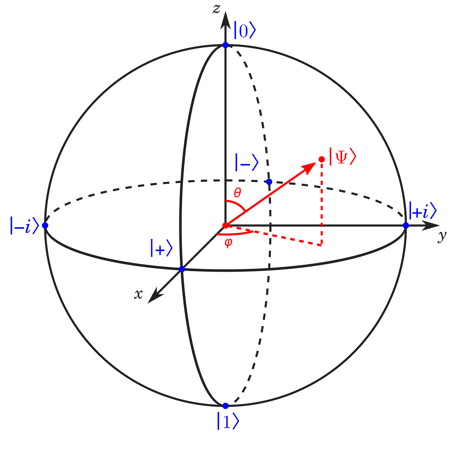The z-axis corresponds to the probability in being measured in $|0\rangle$ and $|1\rangle$. X-axis and y-axis also corresponds to being measured in $|+\rangle$, $|-\rangle$, $|+i\rangle$, and $|-i\rangle$ respectively.

info

$$|+\rangle = \frac{1}{\sqrt{2}}(|0\rangle + |1\rangle)$$$$|-\rangle = \frac{1}{\sqrt{2}}(|0\rangle - |1\rangle)$$$$|+i\rangle = \frac{1}{\sqrt{2}}(|0\rangle + i|1\rangle)$$$$|-i\rangle = \frac{1}{\sqrt{2}}(|0\rangle - i|1\rangle)$$

Quantum circuit gates can be visualized as rotating the state vector (the red arrow) in the bloch sphere. Here are some examples:

1. Pauli-X Gate (NOT Gate):

   • Rotation: $\pi$ radians (180 degrees) around the X-axis.
   • Effect: Transforms the state $|0\rangle$ to $|1\rangle$ and vice versa. On the Bloch sphere, it flips the state from the north pole to the south pole and vice versa.

2. Pauli-Y Gate:

   • Rotation: $\pi$ radians (180 degrees) around the Y-axis.
   • Effect: Applies a complex phase and swaps the states $|0\rangle$ and $|1\rangle$. For example, $|0\rangle$ becomes $i|1\rangle$ and $|1\rangle$ becomes $-i|0\rangle$.

3. Pauli-Z Gate:

   • Rotation: $\pi$ radians (180 degrees) around the Z-axis.
   • Effect: Leaves the state $|0\rangle$ unchanged and adds a phase of $\pi$ (equivalent to a factor of -1) to the state $|1\rangle$.

4. Hadamard Gate (H Gate):

   • Rotation: This gate performs a more complex transformation, equivalent to rotating around the axis at 45 degrees from both X and Z axes, followed by a $\pi$ radian rotation around the Y-axis.
   • Effect: Creates superpositions from basis states, turning $|0\rangle$ into $\frac{|0\rangle + |1\rangle}{\sqrt{2}}$ and $|1\rangle$ into $\frac{|0\rangle - |1\rangle}{\sqrt{2}}$, which is the $|+\rangle$ state.

5. S Gate (Phase Gate):

   • Rotation: $\frac{\pi}{2}$ radians (90 degrees) around the Z-axis.
   • Effect: Leaves the state $|0\rangle$ unchanged and multiplies the state $|1\rangle$ by $i$.

6. T Gate:

   • Rotation: $\frac{\pi}{4}$ radians (45 degrees) around the Z-axis.
   • Effect: Leaves the state $|0\rangle$ unchanged and multiplies the state $|1\rangle$ by $e^{i\pi/4}$, which is a more subtle phase shift than the S gate.

And some parameterized gates:

7. RX Gate:
   • Rotation: $\theta$ radians around the X-axis. It can be represented as a matrix multiplication between the unitary gate matrix and the quantum states, the gate matrix is:

$$R_x(\theta) = \begin{bmatrix} \cos\left(\frac{\theta}{2}\right) & -i\sin\left(\frac{\theta}{2}\right) \\ -i\sin\left(\frac{\theta}{2}\right) & \cos\left(\frac{\theta}{2}\right) \end{bmatrix}$$

8. RY Gate:
   • Rotation: $\theta$ radians around the y-axis:

$$R_y(\theta) = \begin{bmatrix} \cos\left(\frac{\theta}{2}\right) & -\sin\left(\frac{\theta}{2}\right) \\ \sin\left(\frac{\theta}{2}\right) & \cos\left(\frac{\theta}{2}\right) \end{bmatrix}$$

8. RZ Gate:
   • Rotation: $\theta$ radians around the z-axis:

$$R_z(\theta) = \begin{bmatrix} e^{-i\theta/2} & 0 \\ 0 & e^{i\theta/2} \end{bmatrix}$$

And much more.

INFO

Every gate is represented as an unitary gate matrix, e.g. the Hadamard Gate:

$$H = \frac{1}{\sqrt{2}}\begin{bmatrix} 1 & 1 \\ 1 & -1 \end{bmatrix}$$

Also, there are double-qubits gate, for example the CNOT (Controlled-NOT) gate:

$$CNOT = \begin{bmatrix} 1 & 0 & 0 & 0 \\ 0 & 1 & 0 & 0 \\ 0 & 0 & 0 & 1 \\ 0 & 0 & 1 & 0 \end{bmatrix}$$

Controlled gates mean if the first qubit is $|1\rangle$, then the gate (NOT in this case) on second qubit will be performed. There are even triple-qubits gates, like the Toffoli gate (a.k.a. CCNOT), which has a $2^n \times 2^n = 8 \times 8$ size gate matrix.

If you have a quantum states, say 10 qubits, and you want to apply a specific gate on a specific qubit, you can use the Kronecker product to construct a $2^n \times 2^n$ gate matrix and apply it to the quantum states, for example you want to apply the Hadamard gate on the 4th qubit:

$$|\psi_{t+1}\rangle = |\psi_t\rangle \times (I \otimes I \otimes I \otimes \frac{1}{\sqrt{2}}\begin{bmatrix}1 & 1 \\ 1 & -1\end{bmatrix} \otimes I \otimes I \otimes I \otimes I \otimes I \otimes I)$$

tip

$I$ is the identity matrix, i.e. $\begin{bmatrix}1 & 0 \\ 0 & 1\end{bmatrix}$

These quantum gates are crucial in constructing quantum circuits for algorithms, where each type of gate contributes to manipulating the qubit's state in a controlled manner to achieve various computational goals.

Simulation with Qiskit

Qiskit is an open-source framework for quantum computing. It provides the tools for creating quantum circuits, simulating them, and running them on real quantum hardware through IBM's cloud services.

Setting Up Your Environment

To start using Qiskit, make sure Python is installed on your machine, then install Qiskit and Qiskit Aer, which includes simulators that run on your local machine.

pip install qiskit qiskit-aer pylatexenc

Single Qubit Operations

Building the Circuit

We'll begin with a basic single-qubit circuit to demonstrate sequential gate operations that include rotations and a phase shift.

from qiskit import QuantumCircuit, transpile
from qiskit_aer import Aer
from qiskit.visualization import plot_bloch_multivector

# Initialize a Quantum Circuit with 1 qubit
qc_single = QuantumCircuit(1)

# Apply rotation around the X-axis
qc_single.rx(3.14159 / 4, 0)  # Pi/4 rotation

# Apply rotation around the Y-axis
qc_single.ry(3.14159 / 2, 0)  # Pi/2 rotation

# Apply a Z gate
qc_single.z(0)

# Visualize the circuit
print("Single Qubit Circuit:")
print(qc_single.draw(output='mpl'))

Calculating the Expected State Vector

The state vector undergoes a rotation by $\pi/4$ radians around the X-axis, followed by $\pi/2$ around the Y-axis, and finally, a phase shift due to the Z gate.

Simulation and Output

# Prepare the simulator
simulator = Aer.get_backend('statevector_simulator')

# Transpile the circuit for the simulator
transpiled_qc = transpile(qc_single, simulator)

# Run the simulation
job = simulator.run(transpiled_qc)
result = job.result()

# Get the final state vector
statevector = result.get_statevector()
print(statevector)

# Plot the state on the Bloch sphere
plot_bloch_multivector(statevector)

Multi-Qubit Operations

Building the Circuit

We will construct a five-qubit circuit with a combination of entanglement, rotations, and phase shifts to demonstrate the interplay of different quantum gates.

from qiskit import QuantumCircuit, transpile
from qiskit_aer import Aer
from qiskit.visualization import plot_bloch_multivector
from math import pi

# Initialize a Quantum Circuit with 5 qubits
qc_multi = QuantumCircuit(5)

# Apply a Hadamard gate to qubit 0
qc_multi.h(0)

# Apply a CNOT gate between qubit 0 and qubit 1
qc_multi.cx(0, 1)

# Apply a rotation around the X-axis by pi/2 on qubit 1
qc_multi.rx(pi / 2, 1)

# Apply a T gate to qubit 2
qc_multi.t(2)

# Apply a CNOT gate between qubit 1 and qubit 2
qc_multi.cx(1, 2)

# Apply a rotation around the Z-axis by pi/4 on qubit 3
qc_multi.rz(pi / 4, 3)

# Apply a Hadamard gate to qubit 4
qc_multi.h(4)

# Apply a CNOT gate between qubit 4 and qubit 3
qc_multi.cx(4, 3)

# Apply a CNOT gate between qubit 1 and qubit 4
qc_multi.cx(1, 4)

# Visualize the Circuit
print("Five-Qubit Circuit:")
print(qc_multi.draw(output='mpl'))

Calculating the Expected State Vector

Now let's calculate the expected state vector after applying the specified sequence of gates:

1. Initial State
   Operation: All qubits start in $\lvert 00000\rangle$.
   State now:

   $$\lvert 00000\rangle.$$

2. After $H(0)$
   Operation: A Hadamard on qubit 0 creates an equal superposition of $\lvert 0\rangle$ and $\lvert 1\rangle$ (for that qubit).
   State now:

   $$\frac{1}{\sqrt{2}} \bigl(\lvert 00000\rangle + \lvert 10000\rangle\bigr).$$

3. After $\mathrm{CNOT}(0,1)$
   Operation: Qubit 0 is the control, qubit 1 is the target. If qubit 0=1, flip qubit 1.
   State now:

   $$\frac{1}{\sqrt{2}} \bigl(\lvert 00000\rangle + \lvert 11000\rangle\bigr).$$

4. After $\mathrm{RX}\bigl(1,\tfrac{\pi}{2}\bigr)$
   Operation: A rotation by $\theta=\frac{\pi}{2}$ around the $x$‐axis acts on qubit 1. Recall:

   $$R_x\!\Bigl(\tfrac{\pi}{2}\Bigr) \lvert 0\rangle = \tfrac{1}{\sqrt{2}}\bigl(\lvert 0\rangle - i\,\lvert 1\rangle\bigr), \quad R_x\!\Bigl(\tfrac{\pi}{2}\Bigr) \lvert 1\rangle = \tfrac{1}{\sqrt{2}}\bigl(-\,i\,\lvert 0\rangle + \lvert 1\rangle\bigr).$$

   Since the state so far is $\tfrac{1}{\sqrt{2}}(\lvert 00000\rangle + \lvert 11000\rangle)$, applying $\mathrm{RX}(\pi/2)$ to qubit 1 in each term yields four basis states:
   State now:

   $$\frac{1}{2} \Bigl( \lvert 00000\rangle \;-\; i\,\lvert 01000\rangle \;-\; i\,\lvert 10000\rangle \;+\; \lvert 11000\rangle \Bigr).$$

5. After $T(2)$
   Operation: The $T$ gate adds a phase $e^{i\pi/4}$ if qubit 2 is $\lvert 1\rangle$. Here, in all four terms above, qubit 2=$\lvert 0\rangle$, so this gate has no effect.
   State now (unchanged):

   $$\frac{1}{2} \Bigl( \lvert 00000\rangle \;-\; i\,\lvert 01000\rangle \;-\; i\,\lvert 10000\rangle \;+\; \lvert 11000\rangle \Bigr).$$

6. After $\mathrm{CNOT}(1,2)$
   Operation: Qubit 1 is the control, qubit 2 is the target. If qubit 1=1, flip qubit 2.

   • $\lvert 01000\rangle \to \lvert 01100\rangle$.
   • $\lvert 11000\rangle \to \lvert 11100\rangle$.
     State now:
   $$\frac{1}{2} \Bigl( \lvert 00000\rangle \;-\; i\,\lvert 01100\rangle \;-\; i\,\lvert 10000\rangle \;+\; \lvert 11100\rangle \Bigr).$$

7. After $\mathrm{RZ}\bigl(3,\tfrac{\pi}{4}\bigr)$
   Operation: A rotation by $\tfrac{\pi}{4}$ about $Z$ on qubit 3 adds a phase to the $\lvert 1\rangle$ state of that qubit. However, qubit 3=$\lvert 0\rangle$ for all four terms, so only a global phase results (which can be ignored).
   State now (unchanged up to global phase):

   $$\frac{1}{2} \Bigl( \lvert 00000\rangle \;-\; i\,\lvert 01100\rangle \;-\; i\,\lvert 10000\rangle \;+\; \lvert 11100\rangle \Bigr).$$

8. After $H(4)$
   Operation: A Hadamard on qubit 4 (the rightmost qubit) transforms $\lvert 0\rangle\mapsto(\lvert 0\rangle+\lvert 1\rangle)/\sqrt{2}$. Each existing term with qubit 4=0 splits into two terms.
   State now:

   $$\frac{1}{2\sqrt{2}} \Bigl( \lvert 00000\rangle + \lvert 00001\rangle \;-\; i\,\lvert 01100\rangle - i\,\lvert 01101\rangle \;-\; i\,\lvert 10000\rangle - i\,\lvert 10001\rangle \;+\; \lvert 11100\rangle + \lvert 11101\rangle \Bigr).$$

9. After $\mathrm{CNOT}(4,3)$
   Operation: Qubit 4 is the control, qubit 3 is the target. If qubit 4=1, flip qubit 3.
   State now:

   $$\frac{1}{2\sqrt{2}} \Bigl( \lvert 00000\rangle + \lvert 00011\rangle \;-\; i\,\lvert 01100\rangle \;-\; i\,\lvert 01111\rangle \;-\; i\,\lvert 10000\rangle \;-\; i\,\lvert 10011\rangle \;+\; \lvert 11100\rangle + \lvert 11111\rangle \Bigr).$$

10. After $\mathrm{CNOT}(1,4)$
    Operation: Finally, qubit 1 is the control and qubit 4 is the target. Whenever qubit 1=1, flip qubit 4.
    State now (final):

    $$\frac{1}{2\sqrt{2}} \Bigl( \lvert 00000\rangle \;+\; \lvert 00011\rangle \;-\; i\,\lvert 01101\rangle \;-\; i\,\lvert 01110\rangle \;-\; i\,\lvert 10000\rangle \;-\; i\,\lvert 10011\rangle \;+\; \lvert 11101\rangle \;+\; \lvert 11110\rangle \Bigr).$$

This eight‐term superposition (up to any global phase) is the final state of the five‐qubit system after all gates have been applied.

Simulation and Output

# Prepare the simulator
simulator = Aer.get_backend('statevector_simulator')

# Transpile the circuit for the simulator
transpiled_qc = transpile(qc_multi, simulator)

# Run the simulation
job = simulator.run(transpiled_qc)
result = job.result()

# Get the final state vector
statevector = result.get_statevector()
print(statevector)

# Plot the state on the Bloch sphere
plot_bloch_multivector(statevector)

Tasks you may do

1. Implement Shor's Algorithm for finding the prime factors of an integer.
2. Implement Grover's Algorithm for an unstructured search that finds with high probability the unique input to a black box function that produces a particular output value.