Preparing a Gaussian State in the Symmetrical Domain

Explanation of Our Solution at MIT iQuHACK

Introduction

In this blog post, I will explain the solution of our team to the Classiq track at MIT iQuHACK 2025, including why it works and how it scales.

Gaussian state preparation is essential for simulating physical systems and tackling problems in quantum chemistry, machine learning, and optimization. Gaussian states, characterized by their Gaussian-shaped wavefunctions, are powerful tools for encoding probability distributions and modeling quantum systems.

With the scaling of quantum hardware, achieving efficient and precise Gaussian state preparation could improve the costs of quantum algorithms and enhance impactful applications like option pricing in finance, molecular simulations in quantum chemistry, and data analysis in machine learning, among others.

At the competition, our challenge was to prepare a Gaussian state in the symmetrical domain

$$x \in [-2, 2)$$

using a quantum circuit. The target state is defined as:

$$|x_0\rangle_N = |0\rangle_N \longrightarrow \sum_{x\in \text{domain}} \sqrt{G(x)}\,|x\rangle_N,$$

with

$$G(x) = \frac{\exp(-\lambda x^2)}{\sum_{x'\in \text{domain}} \exp(-\lambda {x'}^2)}.$$

Here, $\lambda$ (represented by EXP_RATE in our code) controls the decay of the Gaussian, and the domain discretization is determined by the resolution variable. Our task was to design a quantum circuit that not only achieves a small mean squared error (MSE) compared to the ideal Gaussian state but also scales efficiently as the resolution increases.

There are of course many solutions to this problem. For example, the easiest way is to first prepare a Gaussian state as an amplitude list of length $2^n$ (where $n$ is the number of qubits or resolution), then encode this list of amplitudes into the state vector using amplitude encoding. However, this method is costly, requiring $\mathcal{O}(2^n)$ complexity in the worst case scenario. Another method might be using Hamiltonian simulation with trotterization to calculate the exponentila part of the Gaussian, although it results in a true Gaussian, it is also pretty costly. Our solution is not perfect — it only approximates the Gaussian to an extent, but this approximation is good enough for the MSE error and most importantly, it scales almost linearly to the resolution or number of qubits, i.e. $\mathcal{O}(n)$ complexity.

Our Solution

Our solution is based on two key steps: first, preparing a state using RY rotations that encodes an exponential factor on each qubit, and second, applying the Quantum Fourier Transform (QFT) to convert that state into one with a Gaussian amplitude distribution.

First Step

When we apply an RY gate with angle $\theta$ to a qubit initially in $|0\rangle$, we obtain

$$\text{RY}(\theta)|0\rangle = \cos\Bigl(\frac{\theta}{2}\Bigr)|0\rangle + \sin\Bigl(\frac{\theta}{2}\Bigr)|1\rangle.$$

info

The unitary gate matrix of the RY gate is $R_y(\theta) = \begin{bmatrix} \cos\left(\frac{\theta}{2}\right) & -\sin\left(\frac{\theta}{2}\right) \\ \sin\left(\frac{\theta}{2}\right) & \cos\left(\frac{\theta}{2}\right) \end{bmatrix}$

In our code, for each qubit indexed by $i$ we set

$$\theta_i = 2\,\arctan\Bigl(e^{-\frac{i^2}{2\sigma^2}}\Bigr),$$

with

$$\sigma = \frac{\text{EXP\_RATE}}{\sqrt{5}}.$$

Thus, for the $i$th qubit,

$$\frac{\theta_i}{2} = \arctan\Bigl(e^{-\frac{i^2}{2\sigma^2}}\Bigr).$$

Using the trigonometric identities $\cos(\arctan(x)) = \frac{1}{\sqrt{1+x^2}}$ and $\sin(\arctan(x)) = \frac{x}{\sqrt{1+x^2}}$, with $x = e^{-\frac{i^2}{2\sigma^2}}$, we find

$$\cos\Bigl(\frac{\theta_i}{2}\Bigr) = \frac{1}{\sqrt{1+e^{-\frac{i^2}{\sigma^2}}}}, \quad \sin\Bigl(\frac{\theta_i}{2}\Bigr) = \frac{e^{-\frac{i^2}{2\sigma^2}}}{\sqrt{1+e^{-\frac{i^2}{\sigma^2}}}}.$$

For large $i$, $e^{-\frac{i^2}{2\sigma^2}}$ is very small, so the amplitude in $|1\rangle$ is approximately

$$\sin\Bigl(\frac{\theta_i}{2}\Bigr) \approx e^{-\frac{i^2}{2\sigma^2}}.$$

By applying these rotations to each of the $n$ qubits, the overall state becomes the tensor product

$$|\psi\rangle = \bigotimes_{i=0}^{n-1}\left(\frac{1}{\sqrt{1+e^{-\frac{i^2}{\sigma^2}}}}|0\rangle_i + \frac{e^{-\frac{i^2}{2\sigma^2}}}{\sqrt{1+e^{-\frac{i^2}{\sigma^2}}}}|1\rangle_i\right).$$

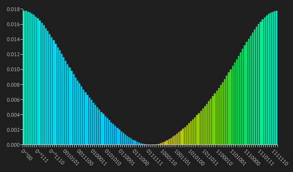
When this state is expressed in the computational basis, a basis state $|j\rangle$ (with $j$ written in binary as $j=\sum_{i=0}^{n-1}j_i2^i$ where each $j_i\in\{0,1\}$) has amplitude

$$a_j = \prod_{i=0}^{n-1}\left[\cos\Bigl(\frac{\theta_i}{2}\Bigr)\right]^{1-j_i}\left[\sin\Bigl(\frac{\theta_i}{2}\Bigr)\right]^{j_i}.$$

Because $\sin(\frac{\theta_i}{2})\approx e^{-\frac{i^2}{2\sigma^2}}$, the amplitude $a_j$ is a product of factors that decay exponentially with $i$. This product structure means that the probability distribution over $j$ appears as a steep exponential drop in the contributions of higher-index qubits rather than as a smooth Gaussian curve. This is shown in the figure below (only the first few amplitudes are shown):

Second Step

The next step is to apply the QFT, which acts on computational basis states as

$$\text{QFT}\,|j\rangle = \frac{1}{\sqrt{N}}\sum_{k=0}^{N-1} e^{2\pi i\,jk/N}\,|k\rangle,$$

with $N=2^n$. After applying the QFT, the final state becomes

$$\text{QFT}\,|\psi\rangle = \sum_{k=0}^{N-1} b_k\,|k\rangle,$$

where

$$b_k = \frac{1}{\sqrt{N}}\sum_{j=0}^{N-1} a_j\,e^{2\pi i\,jk/N}.$$

We can express the sum over $j$ in terms of the binary digits $j_i$. Since $a_j$ is a product over qubit contributions, the sum factorizes, and we have

$$b_k = \frac{1}{\sqrt{N}}\prod_{i=0}^{n-1}\left[\cos\Bigl(\frac{\theta_i}{2}\Bigr) + e^{\frac{2\pi i\,2^ik}{N}}\sin\Bigl(\frac{\theta_i}{2}\Bigr)\right].$$

Substituting the approximate forms for $\cos(\frac{\theta_i}{2})$ and $\sin(\frac{\theta_i}{2})$, this becomes

$$b_k \approx \frac{1}{\sqrt{N}}\prod_{i=0}^{n-1}\frac{1}{\sqrt{1+e^{-\frac{i^2}{\sigma^2}}}}\left[1 + e^{-\frac{i^2}{2\sigma^2}}e^{\frac{2\pi i\,2^ik}{N}}\right].$$

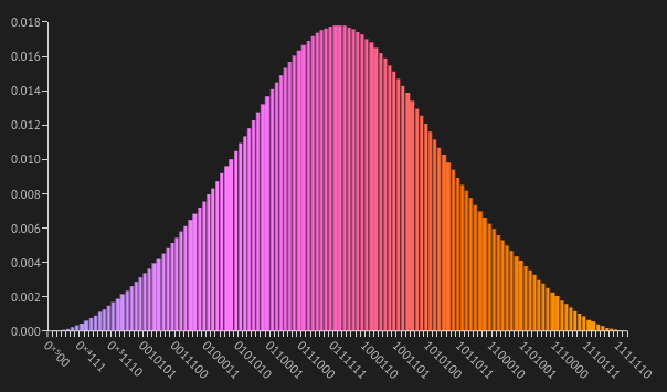
In the large-$N$ limit and with appropriate scaling of $\sigma$, the sum over $j$ approximates the discrete Fourier transform of a Gaussian function. It is a well-known fact that the Fourier transform of a Gaussian is another Gaussian:

$$\int_{-\infty}^{\infty} e^{-\frac{x^2}{2\sigma^2}} e^{2\pi i x k/N}\,dx \propto e^{-2\pi^2 \sigma^2 k^2/N^2},$$

which implies that the amplitudes $b_k$ in the Fourier basis take the form

$$b_k \sim e^{-\alpha k^2},$$

up to normalization and a rescaling of parameters, where $\alpha>0$. Thus, although the original state $|\psi\rangle$ in the computational basis exhibits an exponential decay coming from the product of bitwise factors, the QFT’s property of transforming Gaussians into Gaussians yields a smooth Gaussian distribution in the computational basis after applying QFT. Showing this transformation visually, the amplitudes after QFT are:

Note that the Gaussian is "inverted". To turn it back to a normal Gaussian, we can apply the X gate on the 0th qubit. The final result is:

Using the method described above, we can reach a MSE error of $2.230\times10^{-8}$.

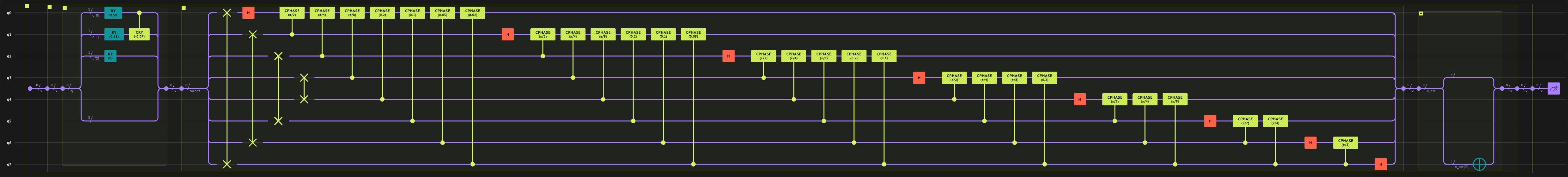
The overall circuit is:

Scalability of Our Solution

The Phase 2 of the challenge is to maximize the scalability of our solution, i.e. make our solution works at the highest resolution with the least number of gates possible. The bottleneck of our solution described above was the QFT part, the number of gates in a regular QFT grows quadratically as the number of qubits increases:

$$\mathcal{O}\left(\frac{n^2+n}{2}\right) \approx \mathcal{O}(n^2).$$

We observed that the gate angles of the CPhase gates used in QFT decreases exponentially! The gate angle for the CPhase gate with layer number $j$ and qubit number $k$ is

$$\frac{2\pi}{2^{k-j+1}}.$$

When there are many qubits, the majority of the gate angles often become very small (e.g. less than $1\times10^{-3}$), which have negligible effects on the overall state vector. Therefore, we pruned any gates with angle smaller than a threshold $\theta$ as shown in the diagram below:

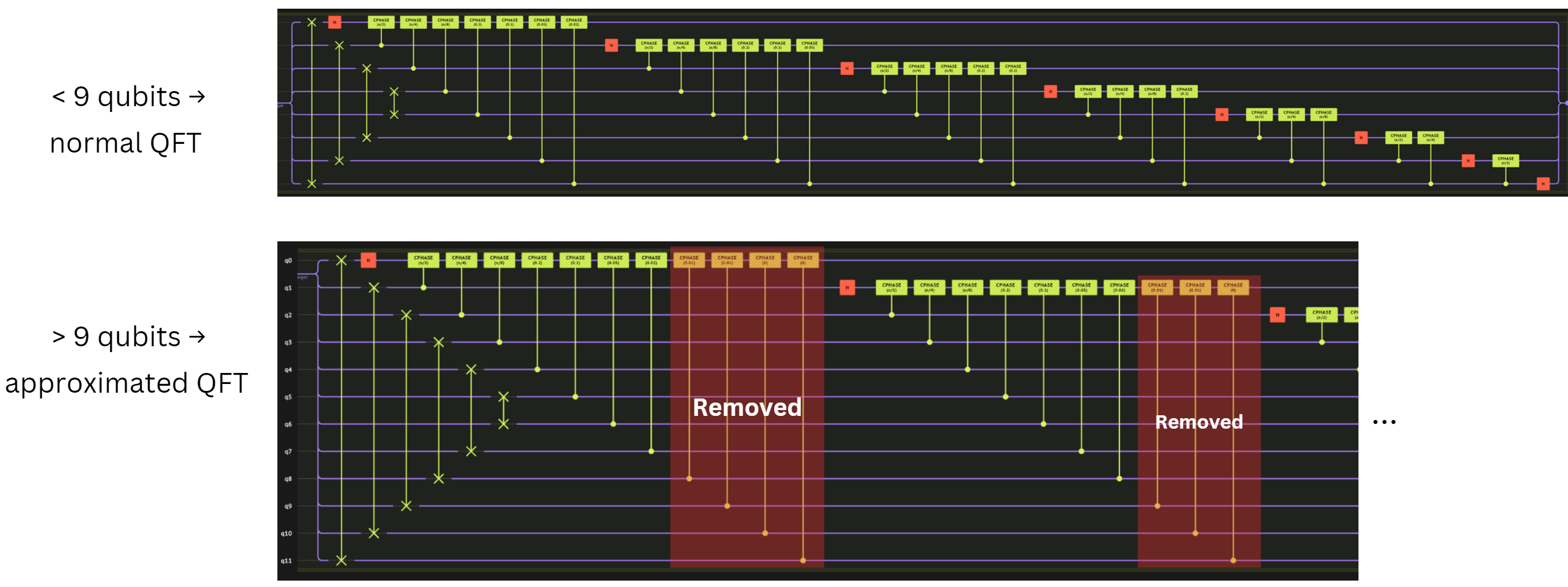
Now the number of gates in the approximated QFT with qubit number $n$ and $\theta=1\times10^{-2}$ is

$$\mathcal{O}\bigl(n+\sum_{j=1}^{n}\text{min}(8,n-j)\bigr) \approx \mathcal{O}(n).$$

We did an experiment to compare the effect of different choices of $\theta$ with 18 qubits (resolution = 18), below is a table summarising the results:

$\theta$	Number of CX Gates	MSE error
$1\times10^{-3}$	293	$1.564\times10^{-14}$
$1\times10^{-2}$	245	$1.601\times10^{-14}$
$1\times10^{-1}$	153	$1.098\times10^{-13}$

We chose $\theta=1\times10^{-2}$ in our final submission for a balance of complexity and accuracy. The figure below shows the ratio between the number of CX gates and the resolution, which can be seen that the relation becomes linear if the resolution is large enough.

Here is an additional table summarising another experiment that compares the difference in MSE error when we change the resolution $n$ from 5 to 18 ($\theta=1\times10^{-2}$):

$n$	Number of CX Gates	MSE error
$5$	28	$2.515\times10^{-5}$
$8$	70	$2.230\times10^{-8}$
$12$	140	$6.526\times10^{-11}$
$15$	191	$1.024\times10^{-12}$
$18$	245	$1.601\times10^{-14}$

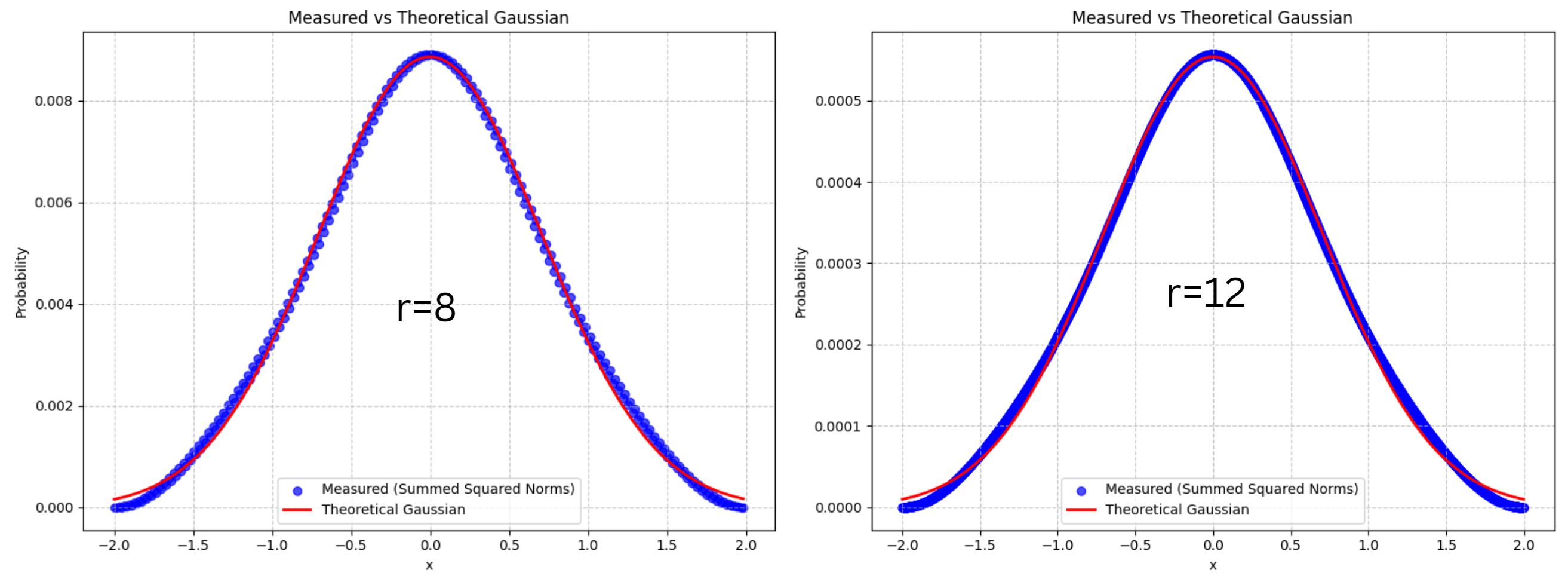
The MSE decreases as the resolution increases. This is because the overall probability scale is smaller when resolution is higher, leading to decreasing MSE. The Gaussian is also more fine-grained as resolution increases, as shown in the following figure:

Code of Our Solution

Below is the code we used for submission. It implements the two-step approach (product-state preparation + approximate QFT) and demonstrates how gate pruning is applied:

def create_solution(resolution: int):
    fraction_digits = resolution - 2
    EXP_RATE = 1
    
    import math
    
    @qfunc
    def single_X(x_arr: QArray[QBit]):
        X(x_arr[0])

    @qfunc
    def prepare_state(q: QArray[QBit]) :
        for i in range(resolution):
            exponent = (i ** 2)/(-2 * (EXP_RATE / math.sqrt(5)) ** 2)
            angle = 2.0 * math.atan(math.exp(exponent))
            if angle > 1e-6:
                RY(angle, q[i])
        CRY(-math.pi/42, q[0], q[1]) # a small "hand-tuned tweak"

    @qfunc
    def approx_qft(target: QArray[QBit]):
        for i in range(resolution // 2):
            SWAP(target[i], target[resolution - i - 1])
            
        for j in range(resolution):
            H(target[j])
            
            for k in range(j+1, resolution):
                theta = 2 * math.pi / (2 ** (k - j + 1))
                if theta > 1e-2: # 9 qubits
                    CPHASE(theta, target[k], target[j])
    
    @qfunc
    def prepare_gaussian(x: QNum):
        prepare_state(x)
        approx_qft(x)
        single_X(x)
        
    return prepare_gaussian

Discussion and Future Work

Our pruning strategy for the QFT threshold $\theta$ was largely heuristic. Further adjusting $\theta$ (either making it adaptive to local circuit conditions or tuning it per qubit layer) may unlock even better trade-offs between gate count and fidelity. An in-depth exploration of different pruning schedules could systematically find the best thresholds for specific MSE targets.

Additionally, while our approach was tested in noiseless simulations, real devices inevitably introduce errors. Testing under realistic noise models (e.g., depolarizing or amplitude-damping channels) will help identify how robust the approximate QFT and the initial product-state preparation are in practice. We plan to run the circuit on a real quantum computer to gauge the impact of gate errors, crosstalk, and qubit decoherence.

Finally, Gaussian states have broad relevance to quantum machine learning (QML), e.g., for encoding continuous data distributions, generating feature maps, or performing kernel-based methods on near-term hardware. A natural next step is to investigate how well our circuit-based Gaussian preparation integrates into QML workflows, particularly in tasks such as clustering or dimensionality reduction. Improved scalability and resilience against hardware noise would make this approach more appealing for real-world QML applications.

Conclusion

We have presented an approach that efficiently prepares a Gaussian state in the symmetrical domain using a circuit of nearly linear complexity. By applying a simple product‐state preparation followed by an approximate QFT with pruning, we achieve a low MSE while keeping the gate count under control. This technique can be extended or refined for many practical tasks that rely on Gaussian states, especially as quantum hardware scales to higher qubit numbers.

Acknowledgements

We thank MIT and Classiq for organizing MIT iQuHACK 2025, and we extend our gratitude to the mentors and judges for their invaluable guidance and support throughout the competition.